Hello everyone! In the first post I shared on modeling NFL game outcomes, I shared a simple way to create a NFL game prediction model using nflreadR and tidymodels. In this post, I’ll share an easy way to tune our model.
I’ll skip the data cleaning portion since it’s the same as the previous post. Ideally, I’d package these steps into a function as part of a larger package to spare you the time and make this process neater, repeatable, and editable. However, I’m not feeling very generous today (aka I’m too lazy), so I’ve copied and pasted the setup code in the hidden cell below.
Code
library('nflreadr')library("tidyverse")library('pROC')library('tidymodels')# Scrape schedule Resultsload_schedules(seasons =seq(2011,2024)) -> nfl_game_results nfl_game_results %>%# Remove the upcoming seasonpivot_longer(cols =c(away_team,home_team),names_to ="home_away",values_to ="team") %>%mutate(team_score =ifelse(home_away =="home_team",yes = home_score,no = away_score),opp_score =ifelse(home_away =="home_team", away_score,home_score)) %>%# sort for cumulative avgarrange(season,week) %>%select(season,game_id,team,team_score,opp_score,week) -> team_gamesteam_games %>%arrange(week) %>%group_by(season,team) %>%# For each team's season calculate the cumulative scores for after each weekmutate(cumul_score_mean =cummean(team_score),cumul_score_opp =cummean(opp_score),cumul_wins =cumsum(team_score > opp_score),cumul_losses =cumsum(team_score < opp_score),cumul_ties =cumsum(team_score == opp_score),cumul_win_pct = cumul_wins / (cumul_wins + cumul_losses),# Create the lag variablecumul_win_pct_lag_1 =lag(cumul_win_pct,1),cumul_score_lag_1 =lag(cumul_score_mean,1),cumul_opp_lag_1 =lag(cumul_score_opp,1) ) %>%# Non-lag variables leak infoselect(week,game_id,contains('lag_1')) %>%ungroup() -> cumul_avgs# Calculate average win pct.team_games %>%group_by(season,team) %>%summarise(wins =sum(team_score > opp_score),losses =sum(team_score < opp_score),ties =sum(team_score == opp_score))%>%ungroup() %>%arrange(season) %>%group_by(team) %>%mutate(win_pct = wins / (wins + losses),lag1_win_pct =lag(win_pct,1)) %>%ungroup() -> team_win_pct# Load depth charts and injury reportsdc =load_depth_charts(seq(2011,most_recent_season()))injuries =load_injuries(seq(2011,most_recent_season()))injuries %>%filter(report_status =="Out") -> out_injdc %>%filter(depth_team ==1) -> starters# Determine roster position of injured playersstarters %>%select(-c(last_name,first_name,position,full_name)) %>%inner_join(out_inj, by =c('season','club_code'='team','gsis_id','game_type','week')) -> injured_starters# Number of injuries by positioninjured_starters %>%group_by(season,club_code,week,position) %>%summarise(starters_injured =n()) %>%ungroup() %>%pivot_wider(names_from = position, names_prefix ="injured_",values_from = starters_injured) -> injuries_positionnfl_game_results %>%inner_join(cumul_avgs, by =c('game_id','season','week','home_team'='team')) %>%inner_join(cumul_avgs, by =c('game_id','season','week','away_team'='team'),suffix =c('_home','_away'))-> w_avgs# Check for stragglersnfl_game_results %>%anti_join(cumul_avgs, by =c('game_id','season','home_team'='team','week')) -> unplayed_games# Indicate whether home team wonw_avgs %>%mutate(home_win =as.numeric(result >0)) -> matchupsmatchups %>%left_join(injuries_position,by =c('season','home_team'='club_code','week')) %>%left_join(injuries_position,by =c('season','away_team'='club_code','week'),suffix =c('_home','_away')) %>%mutate(across(starts_with('injured_'), ~replace_na(.x, 0))) -> matchup_full# Remove unneeded columnsmatchup_full %>%select(-c(home_score,away_score,overtime,home_team,away_team,away_qb_name,home_qb_name,referee,stadium,home_coach,away_coach,ftn,espn,old_game_id,gsis,nfl_detail_id,pfr,pff,result)) -> matchup_ready# Remove columnsmatchup_ready = matchup_ready%>%# Transform outcome into factor variableselect(where(is.numeric),game_id) %>%mutate(home_win =as.factor(home_win))
Long story short, I want each row in the final dataset to represent an NFL game with each team’s :
There are certainly better ways to represent these pieces of information than what I’ve managed to do above (please let me know!), but this post will only focus on the simple step of model tuning.
With that, I’ll start directly from the modeling portion of the code. In the sections below, you’ll see our basic tidymodels setup using our recipes object for pre-processing.
rec_impute =recipe(formula = home_win ~ .,data = train_data) %>%#create ID role (do not remove) game ID. We'll use this to match predictions to specific gamesupdate_role(game_id, new_role ="ID")%>%step_zv(all_predictors()) %>%step_normalize(all_numeric_predictors()) %>%#for each numeric variable/feature, replace any NA's with the median value of that variable/featurestep_impute_median(all_numeric_predictors())
We added an extra step of removing zero-variance predictors.
imp_models <- rec_impute %>%check_missing(all_numeric_predictors()) %>%prep(training = train_data)# Check the predictors that were filtered outnzv_step <- imp_models$steps[[2]] # Access the step_nzv objectremoved_predictors <- nzv_step$removals# Display removed predictorsremoved_predictors
NULL
# Check if imputation workedimp_models %>%bake(train_data) %>%is.na() %>%colSums()
In the last post, we introduced logistic regression as our model of choice. We wanted (and still want) to predict the probability that the home team wins a matchup and do that, we need a classification model.
Enter logistic regression, the simple, yet powerful classification technique made for classifying linear data.
In logistic regression, we have the option of introducing something called regularization, which is just a fancy word for telling the model “don’t overcomplicate things!”. As you saw in the feature enigneering steps in the last post, there are a lot of variables and in many real world models (AI models included) the number of parameters can be in the billions! This is often too much information to pare down, so regularization is a simple step to help the model focus on the most important stuff. This extra step helps the model avoid a common ML pitfall - overfitting. Think of it like this, imagine you have a math test tomorrow and your friend sends you the solutions to the practice exam. You study by memorizing the answers to practce exam (not by DOING the problems). The next day to open your test and … shoot… you have to SHOW your work?? You don’t even know where to start. That is overfitting, you’ve memorized the answers, but you don’t know HOW to solve the problems or complete the process.
Regularization is a way to penalize the model from memorizing inputs and instead forces it to make generalizations about relationships in the data (aka learn general patterns). You sacrifice a bit accuracy, for example, maybe you mix up some calculations on the exam incorrect, but you get partial credit for showing proper process. There are some other pros and cons to regularization, but I’ll leave that for you to research yourself.
Modeling
Also left out in the last post was the crucial step of tuning (or optimizing) those regularization parameters. We fit our model using easy handpicked hand-picked values of mixture = 0.05 and penalty = 1. This time, we’ll try to tune our logistic regression to find the optimal values for both mixture and penalty based on model performance and check if that results in better (and more trustworthy) prediction accuracy. To do that, we introduce two new lines, penalty = tune() and mixture = tune() in the glm_spec variable.
library('glmnet')# Penalized Linear Regressionglm_spec <-logistic_reg(penalty =tune(), mixture =tune() ) %>%set_engine("glmnet")# Setup workflowglm_wflow <-workflow() %>%add_recipe(rec_impute) %>%add_model(glm_spec)# Create cross validation splitsfolds <-vfold_cv(train_data, v =5)# Tune the hyperparameters using a grid of valuesglm_tune_results <-tune_grid( glm_wflow,resamples = folds,metrics =metric_set(brier_class),grid =10# Number of tuning combinations to evaluate)
These 2 lines will incorporate the tuning/optimization into our workflow. To finish the job, we add one more line metrics = metric_set(brier_class) as the evaluation criteria we’re attempting to optimize for. Why we are using brier_class() is explained below.
Brier Score
Next, let’s take a look at the results. We’re primarily concerned with brier score since we want to measure how well our predicted probabilities are calibrated to actual results. Calibration refers to how well the predicted probabilities from a model match the actual observed outcomes. A well-calibrated model means that if it predicts a 70% chance of an event happening, the event should occur about 70% of the time in reality. For example, if a model predicts a team wins 60% of the time, the team should win about 60% of the time.
Brier score is a representation of that calibration on a 0-1 scale. The lower the score, the better Seeing a slight reduction in brier score between the last attempt (0.229) and this attempt (0.216) is good! If we want to go the extra mile, we can test the significance of the difference across CV folds to determine if this reduction is significant.
Looks like the tuning lead us to better model calibration!
# Select the best hyperparameters based on RMSEbest_glm <-select_best(glm_tune_results, metric ='brier_class')# Finalize the workflow with the best hyperparametersfinal_glm_workflow <-finalize_workflow(glm_wflow, best_glm)best_glm
# Fit the finalized model on the entire training datafinal_glm_fit <-fit(final_glm_workflow, data =train_data)
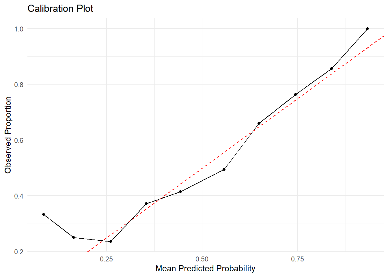
Let’s try out our new evaluation metric to check how well our model is calibrated with the actual output. The graph below is calibration plot. It tells us how aligned our predictions are with the actual observed outcomes. The x-axis is straightforward - it represents our predicted probabilities. The Y-Axis, however, is the proportion of positive observations. This displays our home_win outcome variable as a proportion so we can compare on the scale of the predicted probability class.
It looks like in this case, the model is better calibrated (in-line with actual results) for games between a 50-70% win pct for the home team. This doesn’t tell us much other than that the model is unreliable on the extreme margins, however, NFL games rarely have games with such extreme dogs/favorites.
Regularization and model tuning is just one way to improve model perforance. In the next post, we’ll likely take another crack at improving this model. Thank you for reading and feel free to reach out to me with any questions/suggestions!