Predicting Wide Receiver Fantasy Points w/ Tidymodels Pt 2
Random Intercepts
code
analysis
tidymodels
nfl
Author
Sameer Sapre
Published
May 6, 2025
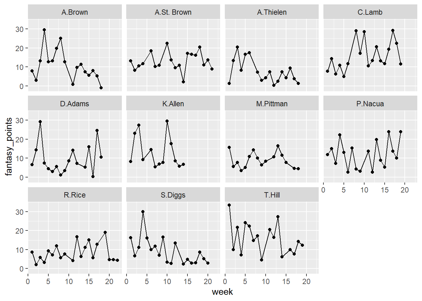
I made a slight mistake. I broke a core assumption of linear regression in the previous edition of the model. To use linear regression, one must assume that each data point is independent of one another. However, this is not the case in the dataset I was working with. Take a look at the sample below. Here are some of the league leaders in receptions for 2023. We can see clearly that we are dealing with some repeated measurements.
Several records exist for each receiver depicted in the plot. This is an example of what scientists call “repeated” measures. It’s a way to describe the process of taking several measurements of a variable on the same subject. This is important because it acknowledges that a core assumption of linear regression is violated (independence) since samples taken or observed from the same subject may not be independent.
In football terms, we want our model to know WHO or WHERE the data is coming from. We want it to know that the data produced by Tyreek Hill is coming from… well… Tyreek Hill. It can be beneficial in this context because it allows us to capture information from our data that may not necessarily be represented by our features (i.e. targets, TDs, yards, etc.)
Let’s take the following example scenario: Dolphins starting QB Tua Tagovailoa has been injured for the past few games, but he is back this week. Hill’s stats haven’t been great with the backup in, but he’s STILL Tyreek Hill. While the basic linear model will just be going off recent week stats, it’s not aware that it’s [TYREEK FREAKING HILL](https://www.youtube.com/watch?v=iPHAUaTlH4w). Acknowledging where the observations come from does that, to an extent.
Now, I’m sure there are probably many nesting structures in the data we’re using. When predicting NFL receiving fantasy points, we can probably nest observations within season, week, team, and/or player. For this exercise, we’ll focus on using player (player_id in the dataset) as the nesting/grouping variable for interpretability. With player_id as our nesting/grouping variable, let’s try to implement this with some familiar code.
# Build a tidymodels recipe object with fantasy points as the targetexp_recipe = train_data %>%recipe(formula = fantasy_points ~ .) %>%update_role(c(recent_team,log_fantasy_points,fantasy_points_ppr,fantasy_points_target),new_role ='ID') %>%add_role(player_id, new_role ="exp_unit") %>%# Impute data with median from each column step_impute_median(all_numeric_predictors()) %>%# Remove zero variance predictors (ie. variables that contribute nothing to prediction)step_zv(all_predictors()) %>%step_center(all_numeric_predictors())
# Calculate the correlation matrix wrt to log fantasy pointscor_matrix <- train_data %>%select(starts_with("wt_"), fantasy_points) %>%cor(use ="complete.obs")cor_data <- reshape2::melt(cor_matrix)# Sort variables by correlation valuecor_data %>%filter(Var1 =="fantasy_points") %>%select(-Var1) %>%arrange(desc(value))
We’re going to train a few simple models, without any regularization, to compare a linear model to a mixed model. This time, we’ll use the workflowsets library from the tidymodels family to combine processes for 2 modeling types (mixed effects and linear models).
library(lme4)
Loading required package: Matrix
Attaching package: 'Matrix'
The following objects are masked from 'package:tidyr':

    expand, pack, unpack
library(multilevelmod)
Warning: package 'multilevelmod' was built under R version 4.4.3
# Create CV folds based on player idplayer_folds <-group_vfold_cv( train_data,group = player_id,v =5)lm_spec <-linear_reg() %>%set_engine("lm")mixed_mod_spec <-linear_reg() %>%set_engine("lmer")# Setup workflow with model formulamixed_wflow <-workflow() %>%add_recipe(exp_recipe) %>%add_model(spec = mixed_mod_spec, formula = fantasy_points ~1+ (1|player_id) + wt_fantasy_points+ wt_wopr + wt_receptions )lm_wflow <-workflow() %>%add_recipe(exp_recipe) %>%add_model(spec = lm_spec,formula = fantasy_points ~ wt_fantasy_points + wt_wopr + wt_receptions)# Create workflow set for easier comparisonmodel_set <-as_workflow_set(linear_model = lm_wflow,mixed_model = mixed_wflow)
In the workflow set defined above, we created a simple linear model consisting of the variables weighted fantasy points, WOPR, and receptions. I wanted to compare this to the mixed effects model which contained a random intercept that varied by the player_id. This is what I mentioned in the section above about taking the player into account in the model.
# Cross Validate across workflow setscv_results <- model_set %>%workflow_map(seed =1502,fn ="fit_resamples",resamples = player_folds,metrics =metric_set(rmse, rsq, mae) )# Collect Metrics and Evaluate Average RMSE across foldscollect_metrics(cv_results, summarize =TRUE) %>%filter(.metric =="rmse")
# A tibble: 2 × 9
  wflow_id     .config      preproc model .metric .estimator  mean     n std_err
  <chr>        <chr>        <chr>   <chr> <chr>   <chr>      <dbl> <int>   <dbl>
1 linear_model Preprocesso… recipe  line… rmse    standard    5.35     5  0.0679
2 mixed_model  Preprocesso… recipe  line… rmse    standard    5.43     5  0.0788
After running the model, the simple linear model actually outperforms the random intercept model according to RMSE. This is not what I expected. Perhaps the nesting structure is incorrect, observations are more independent than they seem, or I have not implemented the mixed model framework correctly. Any way you slice it, we have only really scratched the surface of mixed effect regression models. You can go down a rabbit hole of the random effects (including random coefficiets).
Hat tip to Patrick Ward for the inspiration. Go check out his blog for more Mixed Model content!
Ho T, Carl S (2024). nflreadr: Download ‘nflverse’ Data. R package version 1.4.1.05, https://github.com/nflverse/nflreadr, https://nflreadr.nflverse.com.
Kuhn et al., (2020). Tidymodels: a collection of packages for modeling and machine learning using tidyverse principles. https://www.tidymodels.org
Patrick. (2022, July 11). Mixed Models in Sport Science – Frequentist & Bayesian | Patrick Ward, PhD. Retrieved May 3, 2025, from Optimumsportsperformance.com website: https://optimumsportsperformance.com/blog/mixed-models-in-sport-science-frequentist-bayesian/